


a (very) scenic tour of hnsw
HNSW, which stands for “Hierarchical Navigable Small World” (graphs), is one of the first data structures for which I read not just its paper but (a lot of) the trail of papers backward in time until I arrived at one with a name I already knew. [WIP Post - 01/17/23]
the goal and structure of this tour
I took these notes for myself to capture my own understanding. I think they’re a decent path to retread for others, but if your goal is just to understand how HNSW works or how to use it, I’d sooner recommend Pinecone’s guide.
Because of my background in search, I start with inverted indices to ground and contrast approximate nearest neighbors search. Then I work the name “HNSW” backwards, moving from 1998 through to 2016 when the main paper is published.
my hnsw tl;dr
- We want to query with strictly more expressiveness than exact matching between query and document, so we embed queries and documents into a space where matching is distance.
- We want to calculate distances between our query and our documents as quickly as possible, so we pre-calculate an approximate proximity graph of our documents to each other. It turns out if we rely on random insertion, we can simply save the “garbage” links we produce at the beginning of this graph construction, and our graph actually becomes better for searching efficiently. (This is the navigable small world part.)
- We want to go even faster, so we double down on randomness, but this time via inspiration from skip-lists, and stack proximity graphs from coarse to fine grained. (This is the hierarchical part.)
inverted indices to ann
ANN can be used for different modalities than matching and ranking text documents, but since that’s my main background, I focus on that here.
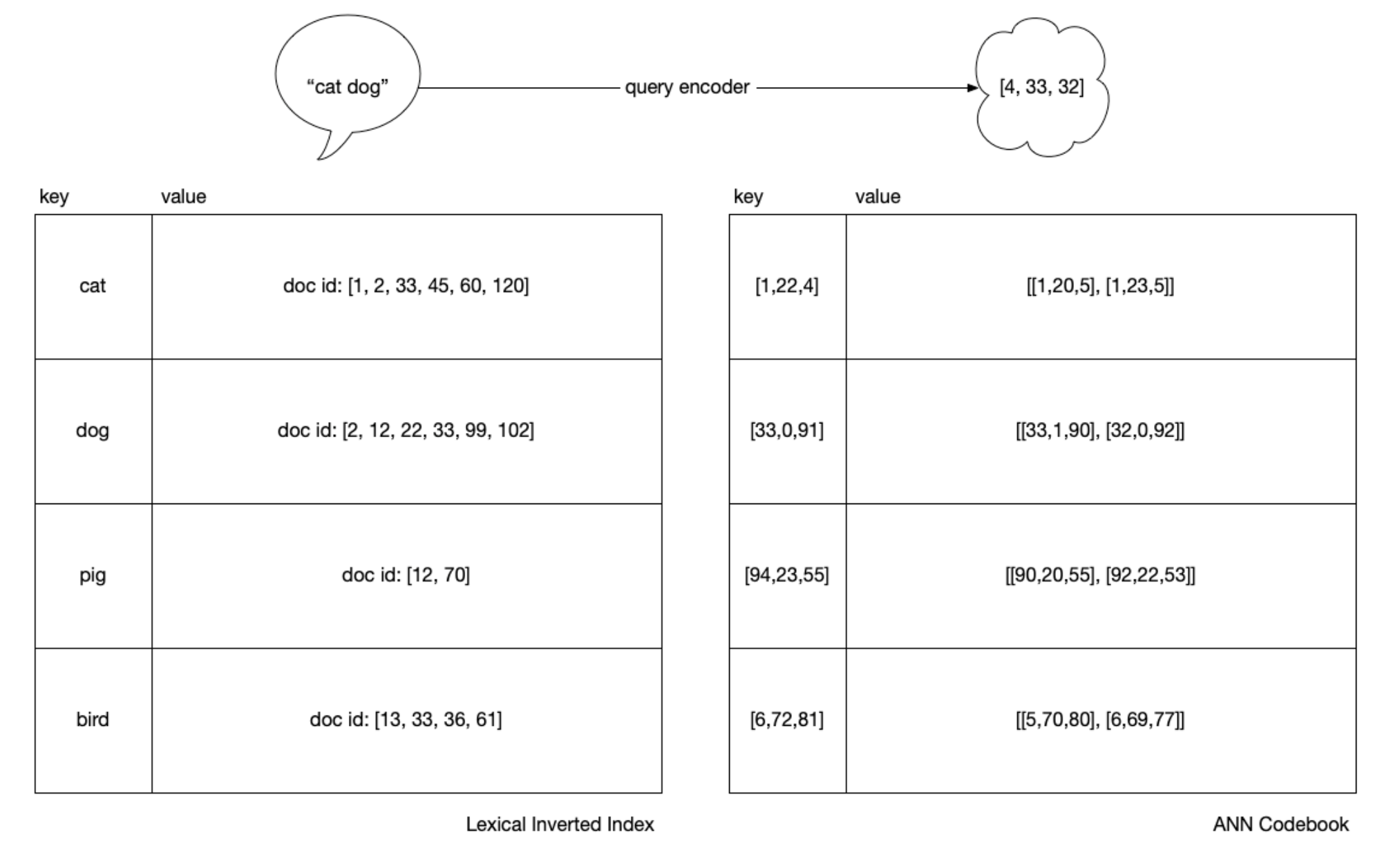
In “lexical” or “sparse” search, documents are tokenized into terms and each term is a key in a dictionary in which we keep some information about the term’s importance in the document. Historically, this information was used to calculate tf-idf or bm25 ranking functions via statistics of the underlying corpus, but it can also be importance information calculated by a deep neural network, as is done in deep impact.
To move to k Nearest Neighbors (KNN) and its approximations, we need to represent our queries and documents differently. Each document has to be encoded into a vector which represents its coordinates in embedding space. A distance function can then measure similarity between documents as closeness in space. Deep neural networks are generally used now to learn this “embedding” vector.
To find the closest documents to a query, we’d need to exhaustively calculate the distance between each. Since this can be slow and expensive at large corpus sizes, it can be worthwhile to construct additional data structures to speed up navigation through the space, which is where HNSW fits in.
For sets in the millions to low tens of millions, it’s common to use HNSW directly. For sets above tens of millions, it’s more common to see clustering applied first, and then HNSW applied to the clusters. In the ANN context, this clustering (whether or not HNSW is employed to speed it up), is called the Inverted File Index or IVF.
a practical aside: ann inverted file format vs inverted indices
As with topic sharding in traditional search, clustering is a technique to trade recall for latency by grouping similar things together and routing the query only to the most “promising” clusters. Commonly we’ll see k-means used for document vectors, then we average each of those clusters to produce averaged “prototype” vectors. If you squint, you can see we use these prototype vectors much like terms in an inverted index.
Although with IVF, we have something “like” an inverted index, an obvious
difference is that we have an added step because we can’t do \(O(1)\) key
lookups since our query does not necessarily equal any prototype or document
vector. With an inverted index, as soon as we have tokenized "cats and dogs"
to ["cat", "dog"] we can use the tokens as keys directly to the lists of
document values, which are called posting lists. In ANN, we must first rank the
cluster prototypes against the query, and only then, for the top clusters, we
rank their members.
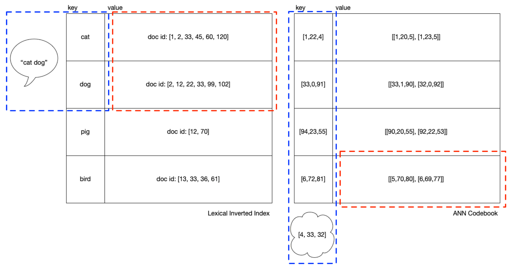
In the below, the “blue box” for ANN is that set of “prototype” vectors representing each of the clusters. To speed up the prototype ranking, we can index the entire “blue box” into an HNSW index.
If you’ve worked with it, you’ve probably noticed many index_factory
settings in
Faiss
start with HNSW, but it can mean more than one thing. If clustering is
being done, they’re laying out how the blue box should be indexed, whereas if
clustering was not done (not pictured) then they’re laying out how all the
embeddings should be indexed.
Looking at the above pictures, you can get some intuition for how you need to
balance the number of clusters (we could say “height” of the IVF) with
balance across the length if the cluster memberships (“width” of the IVF).
Deployments I’ve seen prefer a “long” blue box with an HNSW data structure
to navigate it, signifying many clusters, with relatively “short” red
boxes. k (or efSearch) is the number of top clusters from the blue box
and each of which returns a red box that is scored exactly and
exhaustively. In the runtime, k is tuned to find the best operating
point between recall and latency.
With this structure, it’s possible to serve a lot of embeddings, since the HNSW index of the prototypes can be kept resident in memory, with the cluster member lists memory mapped on disk.
the irl origins of hnsw
Part of what’s fun across the papers leading to HNSW, which I only touch on lightly here and not in the rest of this tour, is that many of them refer to a “real life” phenomenon: the six degrees of separation experiments run by Milgram in the 1960s. If you’re interested in this angle, I’d recommend the first few chapters of Oskar Sandberg’s thesis Searching in a Small World.
Why was it possible that people using only “local” information (who they knew directly) were able to get a message through across a “global” space by a relatively short path a non-negligible amount of the time?
This is actually a very similar question to the one we’re trying to figure out with ANN indexing: if you have a set of \(n\) dimensional points, what information do we need to “navigate” around them quickly?
In fact, it turns out the term “navigable” in “Hierarchical Navigable Small World Graphs” has a precise meaning, as does the mysterious and almost informal sounding “small world.” In order, the title is actually the reverse chronology of the concepts. Since graphs go back to 1736, we’ll skip ahead to the 90s and start with “small world,” just pausing to note the features of graphs needed to understand.
graphs, at sea level
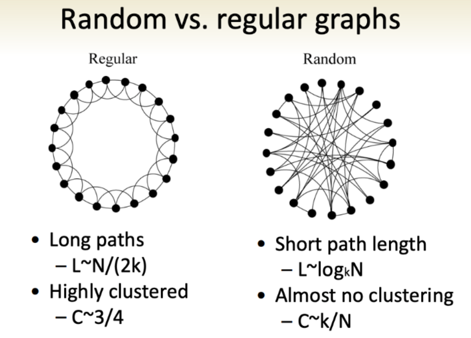
As a simplification, we’ll put graphs on a spectrum. On one end, we have random graphs. On the other end, regular graphs. Beyond the intuitive naming, the graph types can be categorized with a clustering coefficient:
\[C(v)={e(v) \over deg(v)(deg(v)-1)/2}\]where \(e(v)\) denotes the number of edges between the vertices in the \(v\)’s neighbourhood. (The degree [\(deg(v)\)] of a vertex is defined as the number of vertexes in its neighbourhood.)
In other words, the clustering coefficient is the number of edges of a vertex divided roughly by the number of vertices immediately connected to it (ie. \(v\)’s neighborhood). If most of the things connected to you are near you, you’re highly clustered. Regular graphs have this property, while random graphs do not. But at the same time, a regular graph has a high “diameter” (and a random graph low, which Kochen noted was key) because the maximum number of edges in the shortest path connecting the vertices for any vertex is high (or low, if you’re random).
A classic math question, given this and that, is there something in between in a precise and meaningful way? Yes! The small world graph!
1/3rd of the way up, the “small world”
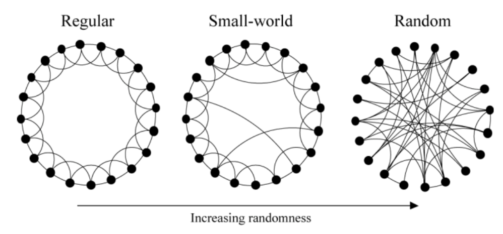
Image from these excellent slides of the Strogatz model of social networks (ring model)
As a sidebar, I was really tickled to find Steven Strogatz worked on this paper since I’ve read some of his books and listened to his podcast. It’s a bit like seeing a celebrity in your local coffee shop.
1998: “Collective dynamics of ‘small-world’ networks”
…these systems can be highly clustered, like regular lattices, yet have small characteristic path lengths, like random graphs.
That is, it turns out with a small world graph you can get a high clustering coefficient but a low diameter, since they have these properties:
most nodes (1) are not neighbors of one another, but the (2) neighbors of any given node are likely to be neighbors of each other and (3) most nodes can be reached from every other node by a small number of hops or steps.
How? Simply by “rewiring” some edges at random! More formally:
With probability \(p\), we reconnect this edge to a vertex chosen uniformly at random over the entire ring, with duplicate edges forbidden; otherwise we leave the edge in place.
Because they can parameterize probability \(p\) between 0 for regular and 1 for random, they’ve found a way to make this or that into a continuous space where there’s a meaningful “between” between.
That parameterization can then allow you to graph the clustering coefficient (\(C(p)\)) and path length (\(L(p)\)), and their relationship, too:
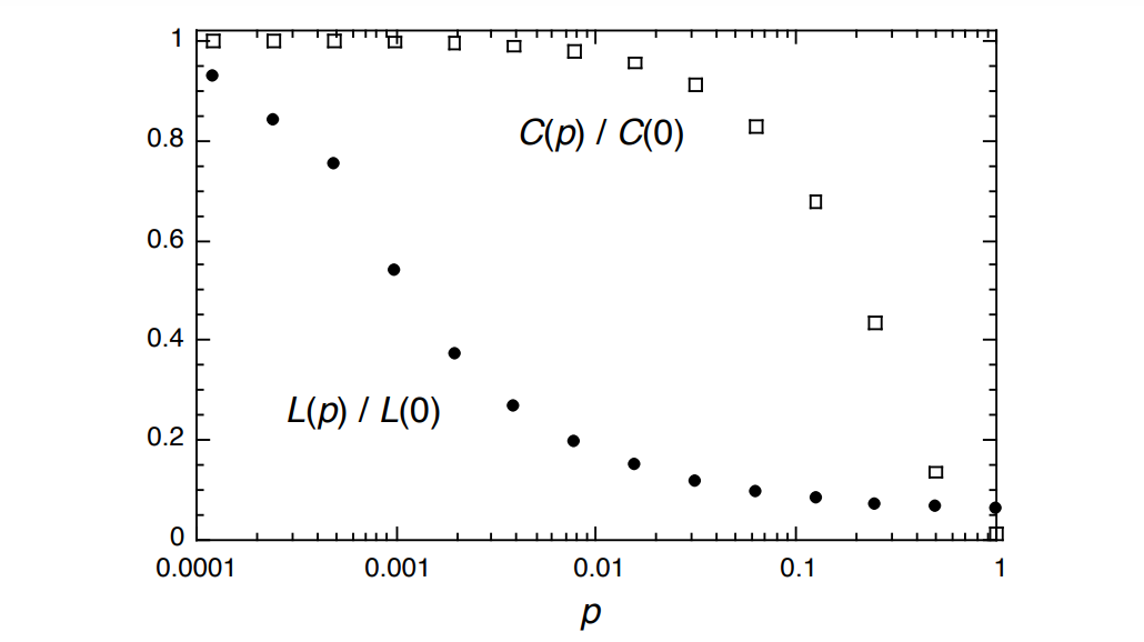
I always love seeing a relatively simple model of a key trade-off. Here it’s the trade-off between clustering and path length.
2/3rds of the way up, navigable
In conversation with Strogatz, Kleinberg picks up and changes the geometry of the question:
Rather than using a ring as the basic structure, however, we begin from a two-dimensional grid and allow for edges to be directed.
This switch from a ring to a lattice (and going from “rewiring” existing edges to adding additional edges) is a generalization that allows him to parameterize the probability with a Manhattan distance.
2000 (May): “The Small-World Phenomenon: An Algorithmic Perspective”
Although recently proposed network models are rich in short paths, we prove that no decentralized algorithm, operating with local information only, can construct short paths in these networks with non-negligible probability. We then define an infinite family of network models that naturally generalizes the Watts-Strogatz model, and show that for one of these models, there is a decentralized algorithm capable of finding short paths with high probability.
Kleinberg’s paper was cited in the 2016 work (it’s further below) that finally began applying these properties to nearest neighbor search with the note:
The first algorithmic navigation model with a local greedy routing was proposed by J. Kleinberg
But funny enough, the word “greedy” doesn’t even appear in this paper. And neither does “navigable”, only “navigation.” That summer though, Kleinberg goes on to write:
2000 (August): “Navigation in a small world”
Where he says directly,
These results indicate that efficient navigability is a fundamental property of only some small-world structures.
In other words, he defines “navigability” as when a “decentralized algorithm can achieve a delivery time [of messages across the network] bounded by any polynomial in \(log(n)\).”
And describes his model that identifies when small worlds will be navigable:
A characteristic feature of small-world networks is that their diameter is exponentially smaller than their size, being bounded by a polynomial in \(log(N)\), where \(N\) is the number of nodes. In other words, there is always a very short path between any two nodes. This does not imply, however, that a decentralized algorithm will be able to discover such short paths. My central finding is that there is in fact a unique value of the exponent \(\alpha\) at which this is possible.
\(\alpha\) is the new parameter for his model, which modifies \(r\), where \(r\) functions as nearly the same long-range connection probability \(p\) Strogatz used. (Again, moving from “rewiring” to adding.)
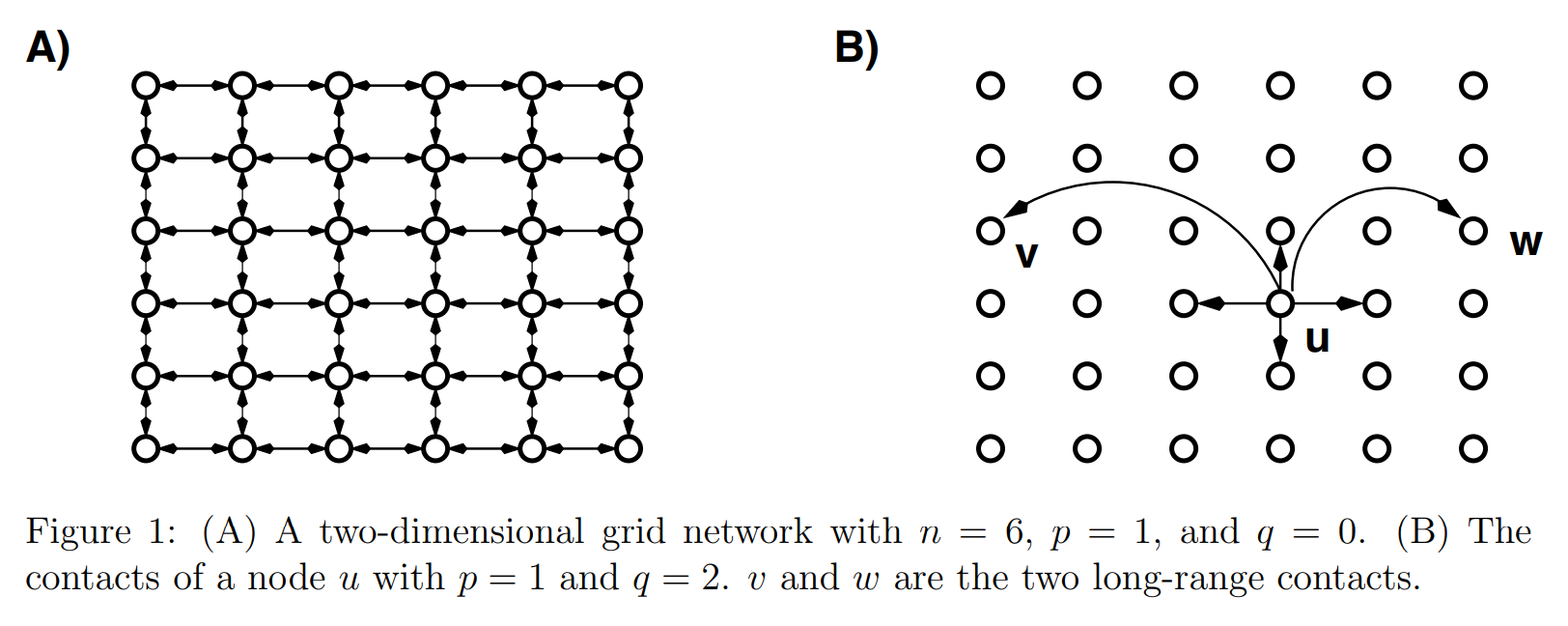
The network model is derived from an \(n \times n\) lattice. Each node, \(u\), has a short-range connection to its nearest neighbours \((a, b, c, d)\) and long-range connection to a randomly chosen node, where node \(v\) is selected with probability proportional to \(r^{1-\alpha}\), where \(r\) is the lattice (“Manhattan”) distance between \(u\) and \(v\).
Or in summary:
Long-range connections are added to a two-dimensional lattice controlled by a clustering exponent, \(\alpha\), that determines the probability of a connection between two nodes as a function of their lattice distance.
He proved for a 2 dimensional lattice \(\alpha=2\), and for a \(d\) dimensional lattice, \(\alpha=d\).
This work was cited a lot in peer-to-peer (P2P) network literature because their essential goal is efficient decentralized access across nodes connected by an overlay network. Depending on how this overlay network is structured, different access patterns may or may not be efficient.
This is from the 2007 paper below. It’s easy to map from overlay network structures being described to graph types:
At one end of the spectrum lie unstructured overlays in which each peer gets connected to a set of arbitrary neighbours. Such networks rely on constrained flooding techniques to search for data. This provides a way to implement all types of search but such approaches often suffer from lack of efficiency. A query may need to ultimately visit the whole network to ensure exhaustive results.
Here you can understand unstructured and “arbitrary” as random, and structured as regular:
Fully structured overlays lie at the other end of the spectrum. In such networks, peers are organized along a precise structure such as a ring. In DHT-based networks, each object gets associated to a given peer. Such networks provide an efficient support for a DHT functionality. However, their expressiveness is naturally limited by the exact-match interface they provide.
brief interlude: proximity graphs
Before we continue through the rest of the papers, I think it’s helpful to zoom back out and visualize what we’re doing. Our question is still how to navigate through \(d\) dimensional points to the closest point to our query.
For simplicity, let’s think about a 2d image for a moment, and consider what pixels are closest to a set of given “seed” pixels. Seed pixels each have a color, and if a point is closest to it, it gets colored the same. To brute force this, we can just go pixel by pixel and calculate its distance to the “seed” pixels. That will produce a Voronoi tessellation:
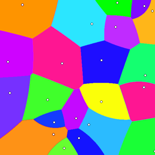
In network overlays or our embedding space though, we are not storing and searching every possible “pixel,” but really just the “seed” ones, and we navigate from one of those to the next. We may get dropped in to any seed to start. If a node only knows about its own nearest neighbors, we’re stuck.
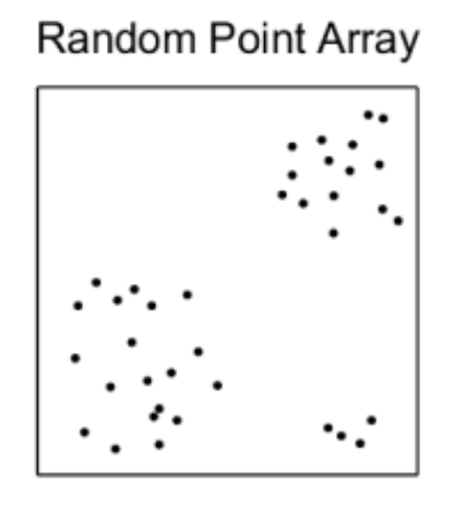
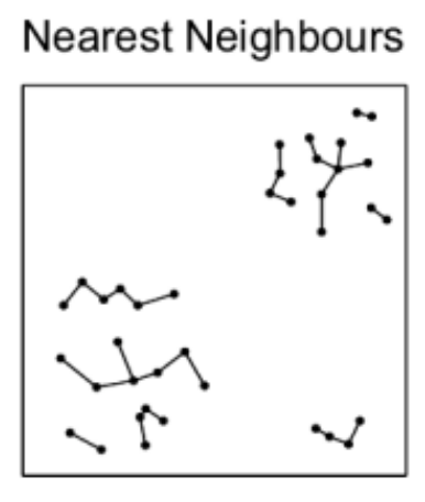
We know we need to add edges between the different nearest neighbor groups, but how? For example, which of the below options works best for search while also allowing for efficient construction?
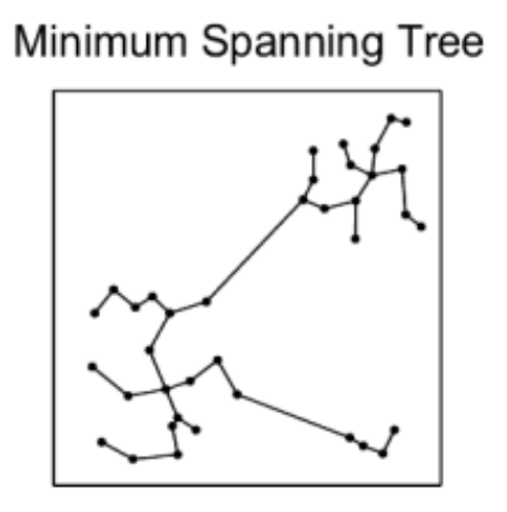
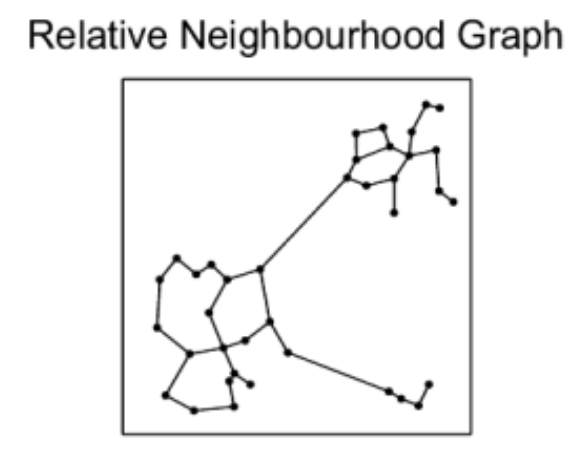
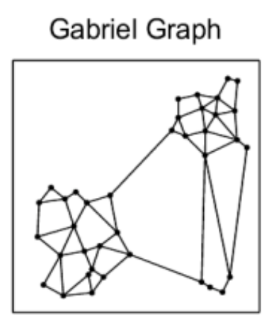
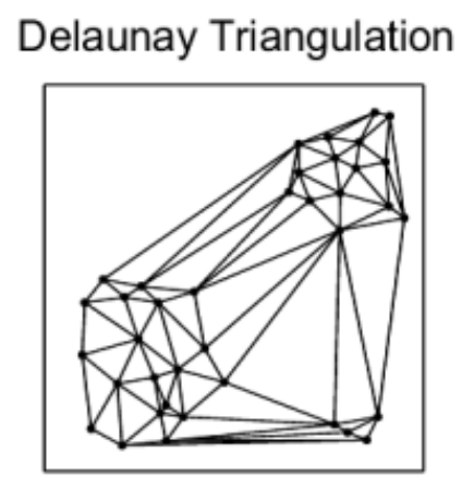
The Delaunay triangulation is dual to the Voronoi tessellation, so we’ll see below first how that got used in the P2P context, then we’ll see how an insight by the authors of HNSW led to an extremely simple approximate construction algorithm which breaks out of P2P entirely.
For a complete survey on the topic of graphs in ANN I found the 2021 paper “A Comprehensive Survey and Experimental Comparison of Graph-Based Approximate Nearest Neighbor Search”.
2006: “VoroNet: A scalable object network based on Voronoi tessellations”
This paper focuses on \(E^2\) and cites Kleinberg’s work on long-range connections, which are tracked in addition to a node’s Voronoi neighbors. Their method for recomputing the Voronoi region is a citation to a paper I couldn’t access, but I assume is exact.
VoroNet [is] an object-based peer to peer overlay network relying on Voronoi tessellations [and] differs from previous overlay networks in that peers are application objects themselves and get identifiers reflecting the semantics of the application instead of relying on hashing functions.
It’s here we actually get something recognizable as an embedding vector, too, just one that isn’t learned:
The overlay design space is a \(d\) dimensional space, each dimension representing one attribute. The coordinates of an object in this space are uniquely specified by its values, one for each attribute.
The authors continue in the Raynet paper, where they pursue an approximation of the Voronoi structure beyond \(E^2\):
2007: “Peer to peer multidimensional overlays: approximating complex structures”
[We] propose the design and evaluation of RayNet, a weakly structured overlay network, achieving an approximation of a Voronoï tessellation. Following the generic approximation method [using Monte-Carlo], each peer in RayNet relies on an epidemic-based protocol to discover its neighbours. Using such a protocol, the quality of the estimation gradually improves to eventually achieve a close approximation of a Voronoï tessellation. […] Each peer in RayNet also maintains a set of long-range links (also called shortcuts) to implement a small-world topology. Efficient (poly-logarithmic) routing in RayNet is achieved by choosing the shortcuts according to a distribution advocated by Kleinberg. Both links are created by gossip-based protocols.
I found these two papers by the next paper (which is actually by the authors of the HNSW paper). Their summary of this work doesn’t mention the gossip-based protocols though, emphasizing instead the Monte-Carlo approximation:
The first structure for solving ANN in \(E^d\) with topology of small world networks is Raynet. It is an extension of earlier work by the same authors Voronet, which solved the problem of the exact NN in \(E^2\). Originally Voronet was envisioned as a p2p network, where every node has coordinates in \(E^2\). In Raynet every node has the coordinates in \(E^d\). The system supports two levels of links - short for correct work of the greedy search algorithm and long - for logarithmic search. Short links correspond to edges of Delaunay graph, i.e. each object has references to objects that are neighbors of its Voronoi region. The main difference of Raynet from Voronet is that in Raynet every object doesn’t know all of its Voronoi neighbors, i.e. Raynet obtains neighborhood with approximately using the Monte Carlo method.
2011: “Approximate Nearest Neighbor Search Small World Approach”
Finally we’ve hit the authors of the eventual HNSW paper, who are responding to the above work:
Raynet is the closest work to ours in terms of general concept. But unlike Raynet, we propose a structure that works with objects from arbitrary metric spaces.
In other words, VoroNet goes from \(E^2\) to Raynet in \(E^d\), while this paper extends beyond \(E\) entirely.
It’s fun to read that 5 years before the “Hierarchical” solution they start from a non-hierarchical one in this paper:
The distinctive feature of our approach is that we build a non-hierarchical structure with possibility of local minimums which are circumvented by performing a series of searches starting from arbitrary elements of the structure.
Which they make precise with (\(m\) is the search attempts):
If probability to find true closest in one search attempt is \(p\) then probability to find the same element in search attempts is \(1-(1-p)^m\), so failure probability decreases exponentially with the number of search attempts.
They do this because:
it is impossible to determine [the] exact Delaunay graph (excluding the variant of the complete graph) [so] we cannot avoid the existence of local minimums [unless we start from multiple random origin points]
One dead-end I had here is that this paper cites two papers I couldn’t find online for how they conceived of the Delaunay construction algorithm, in 2008: “Metrized Small World Properties Data Structure” and in 2009: “Single-attribute Distributed Metrized Small World Data Structure.” That’s too bad because it means I’m not sure how far back to date the key insight (more on it in the two papers below), but they mention it wasn’t new to them in 2011:
In [the 2008 paper and 2009 paper the] authors also have shown theoretically and confirmed by experimental results that graph which constructed by proposed algorithm has properties of small world network if elements arrive in random order.
This is really the big insight of their work that leads eventually to HNSW. This 2011 paper is not cited by the authors, instead the next 2012 paper seems to rewrite this one, with some more plots, and get cited thereafter.
2012: “Scalable Distributed Algorithm for Approximate Nearest Neighbor Search Problem in High Dimensional General Metric Spaces”
The description of construction (adding nodes) is a bit tighter here, so I’ll focus on the key insight here and in the next paper, though it pre-dates this publication:
We propose to assemble the structure by adding elements one by one and connecting them on each step with the \(k\) [NB. this parameter eventually becomes
M] closest objects which are already in the structure. It is based on the idea that intersection of the set of elements which are Voronoi neighbors and the \(k\) closest elements should be large. […] A graph created by such algorithm with data arriving in random order has small world navigation properties without any additional algorithms. That allows us to fully concentrate on the short-range links which approximate the Delaunay graph.
That is, to construct a new node, we basically do a greedy search of the existing nodes. “Hmm,” you might say here, “isn’t that bad? Won’t that mean our initial set of links include some that can’t possibly be nearest?”
Somewhere in here something really clever happened: they realized that when constructing the Delaunay graph randomly like this, the fact that some long-range links are created at the beginning that don’t represent the actual nearest neighbors is good because they’re exactly the kind of shortcuts we want to be a small world!
2013: “Approximate nearest neighbor algorithm based on navigable small world graphs”
Having read the fairly complex methods in the VoroNet and Raynet papers, seeing just how simple this solution ultimately was really felt elegant to me:
The navigable small world is created simply by keeping old Delaunay graph approximation links produced at the start of construction.
I can’t get over this. They basically noticed that they could get exactly what they wanted, for free, by doing it the simple way. “One man’s trash is another man’s treasure.”
Parameters are named somewhat differently at this point but are recognizable:
The parameter \(w\) [NB. this parameter eventually becomes
efConstruction] affects how accurate is determination (recall) of nearest neighbors in the construction algorithm [2012 paper above]. Like in Section 4.2, setting \(w\) to a big number is equivalent to exhaustive search of the closest elements in the structure resulting in a perfect recall.
2016: “Growing Homophilic Networks Are Natural Navigable Small Worlds”
This paper was published in PLOS ONE, which is not a math or CS journal, but general science, and links back to some real-life examples of navigability. (And originally in Physics arXiv 2015.) As it’s targeting a different audience, it has a lot more connection to empirical results. They were clearly trying to see whether the observation they had in previous papers about how to efficiently grow their graphs was getting used by reality somewhere.
In this work we show that [navigability] can be directly achieved by using just two ingredients that are present in the majority of real-life networks: network growth and local homophily, giving a simple and persuasive answer to the question of the nature of navigability in real-life systems.
They define “Growing Homophilic” networks or GH networks as those that are constructed the way they constructed their Delaunay graph in the previous papers but “slightly modified by adding a preferential attachment” to better match observations.
It’s really neat to see the back and forth relationship from observing reality through to pretty abstract concerns in P2P networks all the way back to trying to predict observations about living systems.
the summit: adding hierarchy
We’ve spent like 15 years just in navigability of small worlds!
Though I think arguably the authors had basically everything they needed in 2011 (maybe even 2008) except for the idea of a skip-list to replace the multi-search approach, it’s not until 2016 that we finally see the HNSW paper appear.
I have to mention here that I was introduced to Bill Pugh’s work first through wrestling with getting Fortify and FindBugs to work in an internal build system before learning about his 1990 paper introducing skip-lists. That paper is considerably more fun.
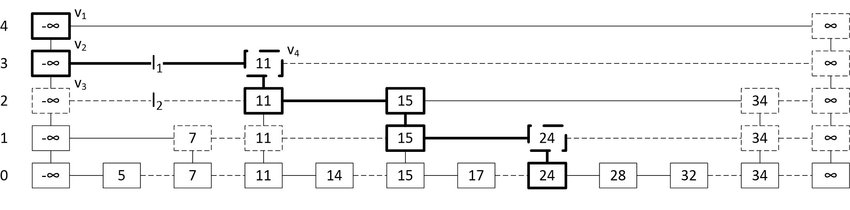
If you’re not familiar
skip-lists, which are
essentially a probabilistic alternative to trees, a picture can help you
see how their hierarchy works to speed up search. In this example, we’re
searching for the leaf node 24 by comparing with elements in “express
lanes” that are randomly sampled sub-lists of the list “lanes” or “levels”
directly below them.
2016: “Efficient and robust approximate nearest neighbor search using Hierarchical Navigable Small World graphs”
(Note: The paper was initially published in 2016, with revisions up to 2018.)
Hierarchical NSW incrementally builds a multi-layer structure consisting from hierarchical set of proximity graphs (layers) for nested subsets of the stored elements.
The HNSW hierarchy is layers of proximity graphs rather than layers of lists, so it looks like this:

The paper compares against many other implementations in ann-benchmarks.com. I perceive now (2022/2023) that Faiss is almost synonymous with its own HNSW implementation, but at the time the benchmark compared HNSW to Faiss’s Inverted Multi-Index (“IMI”).
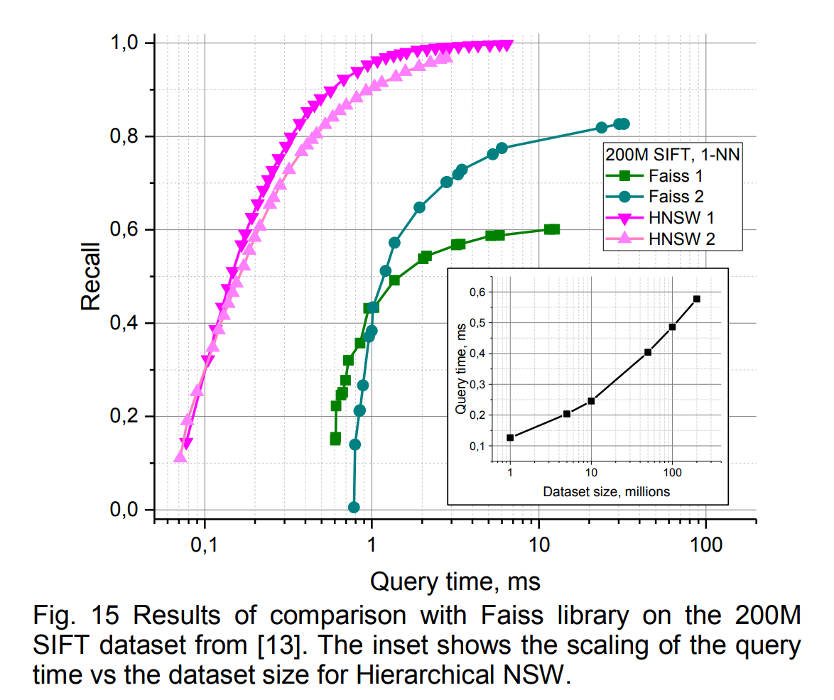
Given that IMI is using quantization, it’s very impressive how much faster HNSW is while also gaining recall. Typically you do expect removing quantization to help recall, but also to slow things down. Knowing what I know now about ANN, I can imagine how exciting this paper was to read when it came out.
HNSW was also much faster than NSW.
The distinctions from NSW (along with some queue optimizations) are: 1) the enter point is a fixed parameter; 2) instead of changing the number of multi-searches, the quality of the search is controlled by a different parameter
ef(which was set toKin NSW).
The construction algorithm takes on new parameters that extend \(M\) (how many nearest neighbors a node is connected to) to per layer values:
The maximum number of connections that an element can have per layer is defined by the parameter \(M_{max}\) for every layer higher than zero (a special parameter \(M_{max0}\) is used for the ground layer separately).
What maximum layer/level a node (embedding) appears in is \(l\) which:
is randomly selected with an exponentially decaying probability distribution (normalized by the \(m_L\) parameter)
This parameterization yields some recognizable forms at minimum and maximum values:
Algorithm construction parameters \(m_L\) and \(M_{max0}\) are responsible for maintaining the small world navigability in the constructed graphs. Setting \(m_L\) to zero (this corresponds to a single layer in the graph) and \(M_{max0}\) to \(M\) leads to production of directed k-NN graphs with a power-law search complexity well studied before (assuming using the alg. 3 for neighbor selection). Setting \(m_L\) to zero and \(M_{max0}\) to infinity leads to production of NSW graphs with polylogarithmic complexity. Finally, setting \(m_L\) to some non-zero value leads to emergence of controllable hierarchy graphs which allow logarithmic search complexity by introduction of layers (see the Section 3).
That is, \(m_L\) at some “in between” value gives us HNSW. They go on to motivate their choice for the optimal value:
A simple choice for the optimal \(m_L\) is \(1/ln(M)\), this corresponds to the skip list parameter \(p=1/M\) with an average single element overlap between the layers.
They note the “only meaningful construction parameter left for the user is
\(M\)” to tune recall. They note it “also defines the memory consumption
of the algorithm (which is proportional to \(M\)), so it should be
selected with care.” But I found this section slightly confusing because
in the next paragraph they mention efConstruction, which is also exposed
to the user. What’s the difference? \(M\) is the number of links formed
between nodes, while efConstruction is the “size of the dynamic
candidate list” in INSERT. Consider that you might want to keep a long
candidate list as you explore, but ultimately only store a top subset of
that as links.
If you’ve only ever used HNSW at runtime, not indexing, you may be
confused that the word efSearch doesn’t appear in this paper. Instead
just ef appears, like efConstruction defined as the “size of the
dynamic candidate list,” here parameterizing the K-NN-SEARCH algorithm.